How to Read Step Output in R
Quick Guide: Interpreting Simple Linear Model Output in R
Linear regression models are a primal office of the family unit of supervised learning models.
13 mins reading fourth dimension 
Linear regression models are a cardinal part of the family of supervised learning models. In particular, linear regression models are a useful tool for predicting a quantitative response. For more details, cheque an article I've written on Unproblematic Linear Regression - An example using R. In general, statistical softwares have different ways to bear witness a model output. This quick guide will assist the analyst who is starting with linear regression in R to sympathise what the model output looks like. In the case beneath, we'll utilise the cars dataset found in the datasets package in R (for more details on the package y'all tin can telephone call: library(help = "datasets").
## speed dist ## Min. : iv.0 Min. : 2.00 ## 1st Qu.:12.0 1st Qu.: 26.00 ## Median :15.0 Median : 36.00 ## Hateful :15.iv Mean : 42.98 ## 3rd Qu.:19.0 tertiary Qu.: 56.00 ## Max. :25.0 Max. :120.00 The cars dataset gives Speed and Stopping Distances of Cars. This dataset is a data frame with fifty rows and 2 variables. The rows refer to cars and the variables refer to speed (the numeric Speed in mph) and dist (the numeric stopping distance in ft.). As the summary output to a higher place shows, the cars dataset's speed variable varies from cars with speed of four mph to 25 mph (the information source mentions these are based on cars from the '20s! - to detect out more than about the dataset, y'all can type ?cars). When it comes to distance to stop, there are cars that can end in 2 feet and cars that demand 120 anxiety to come to a stop.
Below is a scatterplot of the variables:
plot ( cars , col = 'blue' , pch = twenty , cex = 2 , chief = "Relationship between Speed and Stopping Distance for 50 Cars" , xlab = "Speed in mph" , ylab = "Stopping Distance in feet" ) 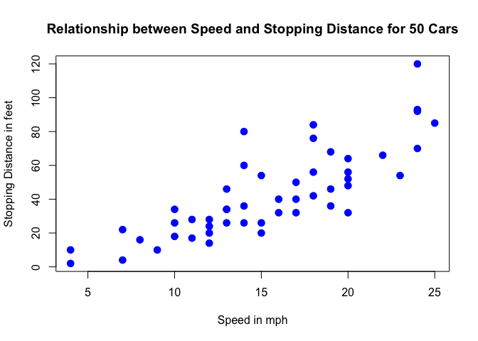
From the plot above, we can visualise that there is a somewhat stiff relationship betwixt a cars' speed and the distance required for information technology to terminate (i.east.: the faster the car goes the longer the altitude it takes to come up to a end).
In this practice, nosotros volition:
- Run a simple linear regression model in R and distil and translate the key components of the R linear model output. Note that for this instance we are not likewise concerned nearly actually fitting the best model merely we are more interested in interpreting the model output - which would then let us to potentially define next steps in the model building process.
Allow's get started by running one case:
gear up.seed ( 122 ) speed.c = scale ( cars $ speed , eye = TRUE , calibration = Simulated ) mod1 = lm ( formula = dist ~ speed.c , information = cars ) summary ( mod1 ) ## ## Phone call: ## lm(formula = dist ~ speed.c, data = cars) ## ## Residuals: ## Min 1Q Median 3Q Max ## -29.069 -nine.525 -2.272 nine.215 43.201 ## ## Coefficients: ## Approximate Std. Error t value Pr(>|t|) ## (Intercept) 42.9800 two.1750 nineteen.761 < 2e-16 *** ## speed.c 3.9324 0.4155 9.464 i.49e-12 *** ## --- ## Signif. codes: 0 '***' 0.001 '**' 0.01 '*' 0.05 '.' 0.1 ' ' one ## ## Residual standard error: xv.38 on 48 degrees of freedom ## Multiple R-squared: 0.6511, Adjusted R-squared: 0.6438 ## F-statistic: 89.57 on 1 and 48 DF, p-value: ane.49e-12 The model above is achieved past using the lm() part in R and the output is chosen using the summary() function on the model.
Below we define and briefly explain each component of the model output:
Formula Call
As y'all can come across, the beginning detail shown in the output is the formula R used to fit the information. Notation the simplicity in the syntax: the formula just needs the predictor (speed) and the target/response variable (dist), together with the data beingness used (cars).
Residuals
The side by side particular in the model output talks about the residuals. Residuals are essentially the difference between the bodily observed response values (altitude to stop dist in our example) and the response values that the model predicted. The Residuals section of the model output breaks information technology downward into 5 summary points. When assessing how well the model fit the data, you should look for a symmetrical distribution beyond these points on the mean value zero (0). In our case, we tin run across that the distribution of the residuals practice not announced to be strongly symmetrical. That ways that the model predicts certain points that fall far away from the actual observed points. We could take this further consider plotting the residuals to see whether this normally distributed, etc. but volition skip this for this case.
Coefficients
The next section in the model output talks nigh the coefficients of the model. Theoretically, in simple linear regression, the coefficients are ii unknown constants that stand for the intercept and slope terms in the linear model. If we wanted to predict the Distance required for a motorcar to finish given its speed, we would get a training set and produce estimates of the coefficients to then use it in the model formula. Ultimately, the analyst wants to find an intercept and a slope such that the resulting fitted line is as close every bit possible to the 50 data points in our data set.
Coefficient - Estimate
The coefficient Approximate contains two rows; the first one is the intercept. The intercept, in our instance, is essentially the expected value of the altitude required for a automobile to end when nosotros consider the average speed of all cars in the dataset. In other words, it takes an boilerplate car in our dataset 42.98 feet to come to a terminate. The 2d row in the Coefficients is the slope, or in our example, the effect speed has in distance required for a motorcar to stop. The slope term in our model is maxim that for every 1 mph increase in the speed of a car, the required altitude to stop goes up by iii.9324088 feet.
Coefficient - Standard Error
The coefficient Standard Error measures the average corporeality that the coefficient estimates vary from the actual average value of our response variable. Nosotros'd ideally desire a lower number relative to its coefficients. In our example, we've previously adamant that for every one mph increment in the speed of a car, the required distance to cease goes upwards by 3.9324088 feet. The Standard Fault can be used to compute an estimate of the expected divergence in instance we ran the model again and again. In other words, we tin say that the required altitude for a car to finish can vary by 0.4155128 feet. The Standard Errors tin can likewise be used to compute confidence intervals and to statistically test the hypothesis of the existence of a relationship between speed and distance required to end.
Coefficient - t value
The coefficient t-value is a measure of how many standard deviations our coefficient guess is far away from 0. We want information technology to be far away from zero as this would point nosotros could reject the null hypothesis - that is, nosotros could declare a relationship between speed and altitude exist. In our case, the t-statistic values are relatively far away from naught and are large relative to the standard error, which could indicate a human relationship exists. In general, t-values are also used to compute p-values.
Coefficient - Pr(>t)
The Pr(>t) acronym plant in the model output relates to the probability of observing whatsoever value equal or larger than t. A small p-value indicates that information technology is unlikely nosotros volition observe a relationship between the predictor (speed) and response (dist) variables due to chance. Typically, a p-value of 5% or less is a practiced cutting-off point. In our model case, the p-values are very close to null. Note the 'signif. Codes' associated to each estimate. 3 stars (or asterisks) represent a highly significant p-value. Consequently, a small p-value for the intercept and the slope indicates that we can reject the cipher hypothesis which allows united states to conclude that there is a relationship between speed and distance.
Residual Standard Error
Residual Standard Error is mensurate of the quality of a linear regression fit. Theoretically, every linear model is assumed to contain an error term Due east. Due to the presence of this error term, we are not capable of perfectly predicting our response variable (dist) from the predictor (speed) i. The Residual Standard Error is the boilerplate amount that the response (dist) will deviate from the true regression line. In our case, the bodily distance required to stop tin deviate from the true regression line past approximately 15.3795867 feet, on boilerplate. In other words, given that the hateful distance for all cars to terminate is 42.98 and that the Residue Standard Error is 15.3795867, nosotros can say that the per centum mistake is (any prediction would still be off past) 35.78%. It's likewise worth noting that the Residual Standard Error was calculated with 48 degrees of freedom. Simplistically, degrees of freedom are the number of information points that went into the estimation of the parameters used after taking into business relationship these parameters (restriction). In our example, we had 50 data points and two parameters (intercept and slope).
Multiple R-squared, Adjusted R-squared
The R-squared ($R^2$) statistic provides a measure of how well the model is plumbing equipment the actual data. It takes the form of a proportion of variance. $R^2$ is a measure out of the linear relationship between our predictor variable (speed) and our response / target variable (dist). Information technology ever lies betwixt 0 and ane (i.due east.: a number well-nigh 0 represents a regression that does not explicate the variance in the response variable well and a number close to 1 does explain the observed variance in the response variable). In our example, the $R^2$ we get is 0.6510794. Or roughly 65% of the variance found in the response variable (dist) can be explained by the predictor variable (speed). Step back and think: If you were able to choose any metric to predict altitude required for a car to terminate, would speed exist one and would it exist an of import one that could help explain how distance would vary based on speed? I guess it'southward easy to see that the respond would almost certainly be a yes. That why we get a relatively stiff $R^2$. Nevertheless, information technology's hard to define what level of $R^2$ is appropriate to merits the model fits well. Essentially, information technology will vary with the application and the domain studied.
A side note: In multiple regression settings, the $R^two$ will e'er increase every bit more than variables are included in the model. That'southward why the adjusted $R^2$ is the preferred mensurate as it adjusts for the number of variables considered.
F-Statistic
F-statistic is a good indicator of whether there is a relationship between our predictor and the response variables. The further the F-statistic is from one the meliorate it is. However, how much larger the F-statistic needs to be depends on both the number of data points and the number of predictors. By and large, when the number of data points is large, an F-statistic that is simply a little bit larger than one is already sufficient to reject the null hypothesis (H0 : There is no relationship between speed and altitude). The contrary is true as if the number of data points is small-scale, a large F-statistic is required to be able to ascertain that in that location may be a human relationship betwixt predictor and response variables. In our instance the F-statistic is 89.5671065 which is relatively larger than 1 given the size of our data.
Annotation that the model we ran to a higher place was just an instance to illustrate how a linear model output looks like in R and how we can start to interpret its components. Obviously the model is not optimised. One way we could beginning to meliorate is by transforming our response variable (try running a new model with the response variable log-transformed mod2 = lm(formula = log(dist) ~ speed.c, data = cars) or a quadratic term and observe the differences encountered). We could too consider bringing in new variables, new transformation of variables then subsequent variable selection, and comparing between dissimilar models. Finally, with a model that is fitting nicely, nosotros could get-go to run predictive analytics to try to estimate distance required for a random car to cease given its speed.
You May Besides Like...
Source: https://feliperego.github.io/blog/2015/10/23/Interpreting-Model-Output-In-R
0 Response to "How to Read Step Output in R"
Post a Comment